1. Hit the ground running : An introductory example
1.1. The model economy
Consider the following 3-equation new Keynesian model (the derivations are available upon request)
The first equation is an (Euler equation) IS curve relating output to the real interest rate.
The second equation is a nonlinear Phillips curve with price adjustment costs.
The third equation is a monetary policy reaction function given by a Taylor-type of rule.
The fourth equation describe the evolution of the cost-push shock process
The fifth equation describes the evolution of the technology shock process.
Where, \(Y_{t}\) denotes output, \(r_{t}\) the gross nominal interest rate (and \(r\) its steady state value), \(\pi _{t}\) inflation (and \(\pi _{\ast }\) the inflation rate targeted by the central bank and \(\pi\) the steady state inflation). \(Z_{t}\) is the technology level. These variables will be referred to as endogenous variables.
In the notation above, we use the convention that uppercase letters denote nonstationary variables and lower-case letters denote stationary variables. This is simply stress the fact that the model is nonstationary and will not be stationarized.
The vector of shocks, known in RISE as exogenous variables, is distributed as
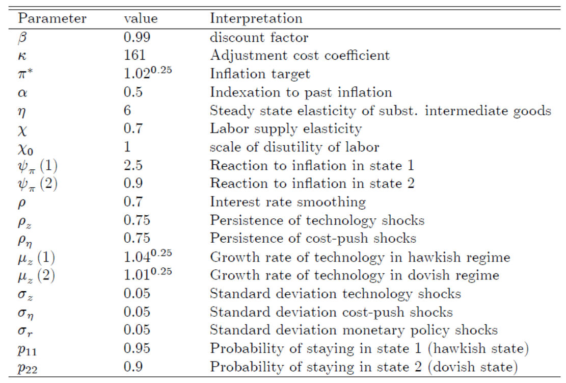
The other elements of the model are parameters, whose description and baseline values are given in the table below. Later on we will demonstrate how to update the values of those parameters via estimation.
We introduce regime switching in the model by assuming — following an example by [Foerster et al., 2016] — that \(\mu _{z}\), the growth rate of the economy, and \(\psi _{\pi }\), the central bank’s reaction to deviation of inflation from its target, are switching in locksteps (This constraint is made simply to keep the example as simple as possible. But it is very easy to relax such an assumption).
We would like to :
Apply a baseline parameterization and solve the model without stationarizing it.
Analyze its dynamics
Estimate the parameters of the model on US data using Bayesian techniques
Such an exercise is straightforward to implement and run in RISE. We will need to
Write down the model equations in a text file with extension rs, rz or dsge
Collect and process the data
Write Matlab instructions for the different tasks.
1.2. Baseline calibration
We consider the following calibration for illustration purposes.
1.3. Preparing the model for RISE
The equations above alongside their variables and parameters can be written in the most natural way in a text file with extension .rs, .rz, .dsge . In this case, we created a file with name “model.rs”.
In the file, although the order is not important, we first declare the various atoms using keywords to announce the type. In particular,
endogenous variables are listed under @endogenous
exogenous variables are listed under @exogenous
parameters are listed under @parameters
We can optionally give a description of each atom using pairs of quote marks. e.g. R is the “interest rate”.
Successive atoms can be separated by a blank spaces, a comma or both.
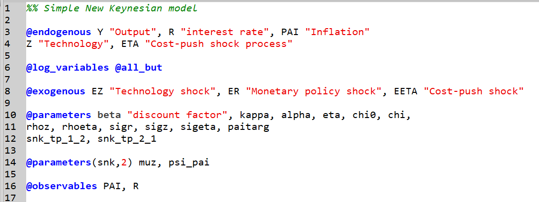
Note that there are two types of parameters. The constant parameters and the switching parameters are declared in different lists.
For the switching parameters, the user must give a name for each Markov process. In the example at hand, we called the process snk and assigned it two states (parameters(snk,2)), and then listed the parameters controlled by the Markov process. Obviously, a parameter cannot belong to more than one list.
Markov processes give rise to transition probabilities, which in the current example are constant over time.
It should be clear by now that in RISE a block starts with a keyword and ends when another keyword appears or when the file ends.
There are two more details worth noting. The @observables declaration simply lists the variables that will be observed in case we conduct a filtration exercise.
The endogenous block uses @endogenous(log) rather than the plain @endogenous keyword. This tells RISE to take a log approximation of every variable listed there. Listing only some of the variables under @endogenous(log) (and the rest under @endogenous) would log just that subset; here we want logs for all five.
The second part of the code lists the model equations. We declare the model equations by issuing keyword @model and there can be many such declarations for the same model. Each equation can be optionally prepended with an equation tag describing the equation. Just like the description of the atoms, the description of the equation tags appears in pairs of quote marks.
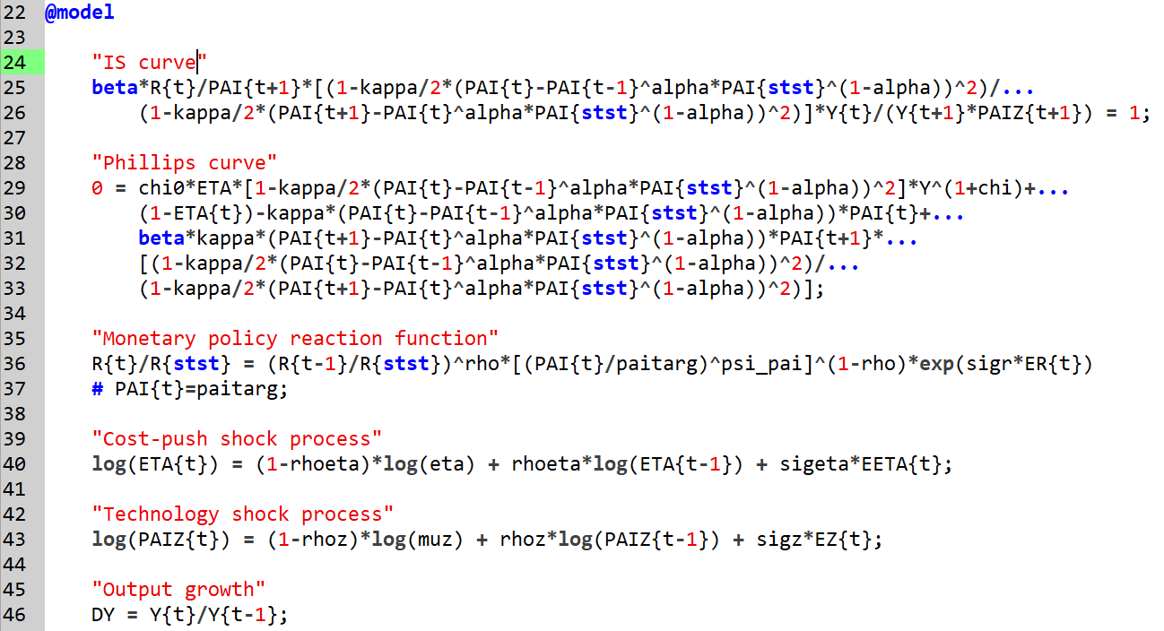
In this example, we choose to denote time using curly braces. RISE would also accept parentheses although in that case it becomes difficult to know whether we are referring to a variable or a function. In any case, stst denotes the steady state.
1.4. Creating the model object (rising the model)
Once the model file is written, we can go ahead an create a rise model object
m=rise('model');
or alternatively a dsge model object
m=dsge('model');
Both classes are isomorphic except that a dsge object is not a rise object.
Without further options, RISE will compute and store in memory, first-order symbolic derivatives suitable for solving a first-order perturbation.
1.5. Parameterizing the model
There are different ways of parameterizing a model. In the code block below, we use a Matlab structure.
p=struct();
p.beta=0.99;
p.kappa=161;
p.paitarg=1.02^0.25;
p.alpha = 0.5;
p.eta = 6;
p.chi = 0.7;
p.chi0 = 1;
p.psi_pai_snk_1=2.5;
p.psi_pai_snk_2=0.9;
p.rho = 0.7;
p.rhoz=0.75;
p.rhoeta=0.75;
p.muz_snk_1=1.04^.25;
p.muz_snk_2=1.01^.25;
p.sigz=0.05;
p.sigeta=0.05;
p.sigr=0.05;
p.snk_tp_1_2=1-0.95;
p.snk_tp_2_1=1-.9;

m=set(m,'parameters',p);
Note how we write the switching parameters : the name of the parameter is followed by an underscore, then the name of the controlling Markov process, then a second underscore, then the state of the Markov process.
1.6. Setting some options for the solution
We could have stationarized the model but we didn’t do so. Here we let RISE know that
the model is nonstationary : solve_bgp =true
We would like to use the Maih-Waggoner perturbation : solve_perturbation_type = ‘mw’
Because we are using the Maih-Waggoner perturbation, we can apply an efficient solver : solver=’dsge_udc’
m=set(m,'solve_perturbation_type','mw',...
    'solve_bgp',true,...
    'solver','dsge_udc');
1.7. Stochastic simulation in a Dynare-like run
Dynare’s keyword and function “stoch_simul” has been overloaded to work with dsge/rise objects. But unlike Dynare’s stoch_simul, RISE’s stoch_simul will not create graphic files and store them. It is the responsibility of the user to collect whatever information he needs in the stochastic simulation structure, called info in the code below, for further processing.
info =stoch_simul(m);

disp(info)
The output structure will contain among other things
simulated data
moments of endogenous variables
impulse responses
autocorrelation of endogenous variables
skewness and kurtosis of endogenous variables
1.8. Solving the model and printing the solution
An alternative way of running rise is to do one thing at a time. In this section we are simply solving the model and printing the policy functions.
By default, the model is solved at first-order of perturbation.
m = solve(m);

print_solution(m)
1.9. Solving a 5th-order perturbation
m5=solve(m,'solve_order',5,...
    'solve_derivatives_type','automatic');

print_solution(m5)
Because we have not instructed RISE to compute symbolic derivatives of order 5, we have two choices:
we can go back and run \(m=rise('model','max\_deriv\_order',5)\) so as to have symbolic derivatives ready or
change the type of derivatives
In the statement above, we opt for automatic (or algorithmic) derivatives. Another choice could have been (finite-difference) numerical derivatives, but they are very imprecise.
1.10. Checking the accuracy of derivatives
check_derivatives(m)
Here we check wether symbolic and numerical derivatives give similar results as automatic derivatives taken to be the most accurate.
1.11. Impulse response functions
myirfs=irf(m);

% plot irfs for the original variables only (exclude auxiliary ones)

quick_irfs(m,myirfs,get(m,'endo_list(original)'))
Here we compute impulse responses. RISE will return the result as a structure of time series
The first level will be the names of the shocks (exogenous variables)
The second level will be the names of the endogenous variables
The irf function just as virtually all functions in the dsge/rise class can be called with options.
1.12. Collecting Data from FRED
Now we want to estimate unobservable variables through filtration and eventually confront the model to the data. In both cases we need observable variables. One way to obtain those variables is to fetch them from the FRED database.
Once the variables we want are fetched, we can transform them so as to relate them to model variables.
Below here, we are selecting the sample to use under filtration, but we do not have to do that at this stage. It can be done during filtration or during estimation.
xrange='1960Q1:2022Q3';

rawdb=fetch_fred({'BPCCRO1Q156NBEA','BOGZ1FL072052006Q','NAEXKP01USQ657S'});

db=struct();

db.PAI=1+rawdb(1).series(xrange)/100;

db.R=1+rawdb(2).series(xrange)/100;

db.GROWTH=1+rawdb(3).series(xrange)/100;
1.13. Filtration
Where we apply the Kalman filter to estimate unobservable variables at the current calibration of the model.
m=set(m,'data',db,...
    'kf_init_variance',1,...
        'kf_presample',10);

f=filter(m);
Before doing that, we set some options. The ‘data’ option does not need any further explanation. However the two other options are there for a purpose :
kf_init_variance = 1 : we set the initial variance for all endogenous variables to 1. This is because the model is nonstationary and therefore does not have a finite variance for all endogenous variables.
kf_presample = 10 : we are burning 10 initial observations that will not be taken into account when computing the likelihood. This is an attempt to amend the fact that we have imposed a finite variance to nonstationary variables.
1.14. Priors for Bayesian estimation
We set priors for Bayesian estimation. In this example we do not set priors in terms of means and standard deviations but rather in terms of quantiles. Of course we could have a mixture in which some priors are set in terms of means and standard deviations and some other set in terms of quantiles. See the next chapter for details.
priors=struct();
priors.kappa={p.kappa,5,20,'gamma(.9)'};
priors.alpha={p.alpha, 0.05,0.948,'beta(.9)'};
priors.chi={p.chi,1.5,3,'gamma(.9)'};

priors.eta={p.eta,3,8,1,12,'beta(.9)'};
priors.muz_snk_1={p.muz_snk_1,1.02^.25,1.05^.25,1,1.07^.25,'beta(.9)'};
priors.muz_snk_2={p.muz_snk_2,1.01^.25,1.03^.25,1,1.04^.25,'beta(.9)'};

priors.rho={p.rho, 0.05,0.948,'beta(.9)'};
priors.rhoz={p.rhoz, 0.05,0.948,'beta(.9)'};
priors.rhoeta={p.rhoeta, 0.05,0.948,'beta(.9)'};

priors.sigz={p.sigz, 0.0005,1.0,'sichisq(.9)',0,3};
priors.sigeta={p.sigeta, 0.0005,1.0,'sichisq(.9)',0,3};
priors.sigr={p.sigr, 0.0005,1.0,'sichisq(.9)',0,3};

priors.snk_tp_1_2={p.snk_tp_1_2, 0.01,0.411,'beta(.9)'};
priors.snk_tp_2_1={p.snk_tp_2_1, 0.01,0.411,'beta(.9)'};

priors.psi_pai_snk_1={p.psi_pai_snk_1, 1.1,2.5,1,3,'beta(.9)'};
priors.psi_pai_snk_2={p.psi_pai_snk_2, 0.5,1.1,0.1,1.5,'beta(.9)'};
1.15. Visualizing the priors
plotOpts=struct();
plotOpts.prior_trunc=2.6e-3;

rdist.plot(priors,plotOpts,[],struct('linewidth',2))
1.16. Posterior maximization
The data were already pushed into the model object while we were doing filtration. All we need now in order to maximize the posterior distribution is prior information and possibly some additional options for tailoring the estimation process.
mest=estimate(m,'estim_priors',priors);
1.17. Posterior simulation
We don’t have to maximize the posterior distribution and use it as a starting point for posterior simulation. However, in this class of models, it is a good practice to do so if we do not have a good posterior sampling procedure.
The posterior samplers in RISE require a starting point and a positive-definite covariance matrix. Again, let’s stress that the starting point need not be the mode of the posterior distribution.
[objective,lb,ub,x0,SIG]=pull_objective(mest);

scale=0.0794;
myOpts=struct();
myOpts.tunedCov=scale*SIG;
myOpts.N=20000;

% Use a maximization objective for sampling
energy=@(varargin)-objective(varargin{:});

results=sample(rsamplers.rwmh(energy,x0,lb,ub,myOpts));
Here we illustrate the basic call to the Random-Walk Metropolis-Hastings algorithm. More options can be added.
Note that objective is a function to be minimized while energy is a function to be maximized.
This is just one out of many possibilities for sampling the posterior distribution in RISE.
1.18. Computation of the marginal data density using the Bridge approach
RISE has 9 ways of computing the marginal data density. Here we illustrate the computation of the marginal likelihood or marginal data density by the method of Meng and Wong (1996).
mddobj=mdd(results,energy,lb,ub,...
        [],[],true);

bridge(mddobj,true,mdd.global_options)